This project focuses on developing and comparing deep learning systems to classify knee MRI images for detecting meniscus tears. The implementation compares a custom Convolutional Neural Network (CNN) with ResNet architecture to distinguish between normal meniscus (“n” label) and torn meniscus (“p” label) in sagittal MRI images from the Stanford University MRNet database.
Research Context
Problem Statement
- Building CNN models to detect meniscus tears from MRI images of the knee
- Training and evaluating performance of custom CNN vs. ResNet model
- Assessment using multiple metrics and hyperparameters
- Addressing class imbalance and optimizing for different clinical goals
Data Source
MRNet database from Stanford University Medical Center
- 5-fold cross-validation structure (.csv files for each process)
- MRI images in sagittal plane with original size 256×256 pixels
- Significant class imbalance (6-7 times more negative cases)
Code Structure and Logic
Task Strategy Flowchart
- Exploratory Data Analysis
- Image Processing and preprocessing
- Parameter definition for model training
- Train CNN & ResNet on each of 5 folds
- Aggregation methods and decision threshold optimization
- Performance metrics assessment
- Data augmentation for best performing models
1. Data Preparation and Setup
Google Drive Integration
The code begins by mounting Google Drive to access the dataset stored in the cloud, creating a working directory, and copying/unzipping the dataset for processing.
Data Organization
The dataset is organized into three main splits:
- Training set: Used to train the model
- Validation set: Used for hyperparameter tuning and model evaluation during training
- Test set: Used for final model evaluation
Each set contains multiple folds for cross-validation, stored as CSV files with image paths and corresponding labels.
2. Data Loading and Exploration
The code identifies all CSV files for training, validation, and testing, then creates dictionaries storing fold information for organized access.
csv_train_files = [filename for filename in os.listdir('dataframe/') if '_train_' in filename]
csv_val_files = [filename for filename in os.listdir('dataframe/') if '_val_' in filename]
csv_test_files = [filename for filename in os.listdir('dataframe/') if '_test_' in filename]

def read_all_images(file_list):
    image_label_df = pd.DataFrame()
    for index, filename in enumerate(file_list):
        temp_df = pd.read_csv('/content/AI-meniscus/dataframe/' + filename)
        image_label_df = pd.concat([image_label_df, temp_df])
    image_label_df.drop_duplicates(inplace = True, ignore_index = True)
    return image_label_df

images_labels_df = read_all_images(csv_train_files)
Data Distribution Analysis
The implementation includes comprehensive analysis of:
# Iterate over each set (train, val, test)
for set_name, folds_dict in [('train', train_folds_dict), ('val', val_folds_dict), ('test', test_folds_dict)]:
    print(f"\n{set_name.upper()} SET:")

    # Iterate over each fold
    for fold, temp_df in folds_dict.items():
        # Get the number of 'n' and 'p' labels in this fold
        num_n_labels = temp_df['label'].value_counts().get('n', 0)
        num_p_labels = temp_df['label'].value_counts().get('p', 0)
        num_images = len(temp_df)

        # Print the counts
        print(f"Fold {fold}:")
        print(f"Number of images: {num_images}")
        print(f"Number of 'n' labels: {num_n_labels}")
        print(f"Number of 'p' labels: {num_p_labels}")
 The resizing of the images of the dataset was essential since it allowed for the CNN to focus only on the image of the knee in order to extract information. By isolating and training the neural networks only on that part of the image, a lot of the noise in the dataset was removed and the efficiency of the CNN increased significantly.
3. Image Preprocessing
import cv2
import os

def create_traintestval_folder(folder_path='./train', folds_dict=train_folds_dict):
    os.makedirs(folder_path, exist_ok=True)

    for fold in folds_dict.keys():
        fold_folder_path = os.path.join(folder_path, fold)
        os.makedirs(fold_folder_path, exist_ok=True)

        temp_df = folds_dict[fold]

        for img_filename in temp_df['img_dir']:
            img = cv2.imread(img_filename)
            height, width = img.shape[:2]

            # Calculate the center of the image
            center_x, center_y = width // 2, height // 2

            # Define the dimensions of the new square
            new_width, new_height = 128, 128

            # Calculate the top-left coordinates for the cropping
            top_left_x = max(center_x - new_width // 2, 0)
            top_left_y = max(center_y - new_height // 2, 0)

            # Ensure the cropping area does not exceed the image dimensions
            if top_left_x + new_width > width:
                top_left_x = width - new_width
            if top_left_y + new_height > height:
                top_left_y = height - new_height

            # Crop the image
            cropped_img = img[top_left_y:top_left_y + new_height, top_left_x:top_left_x + new_width]

            # Save the cropped image
            cv2.imwrite(os.path.join(fold_folder_path, img_filename.replace('images/', '')), cropped_img)

# Takes at least 2:30 minutes
create_traintestval_folder(folder_path = './train', folds_dict = train_folds_dict)
create_traintestval_folder(folder_path = './val', folds_dict = val_folds_dict)
create_traintestval_folder(folder_path = './test', folds_dict = test_folds_dict)
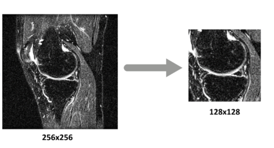
Center Cropping
The preprocessing function extracts 128×128 pixel center crops from original 256×256 images, maintaining anatomical focus on the meniscus region and creating an organized folder structure for processed images.
Preprocessing Benefits
- Dimensionality reduction: Faster training with smaller images
- Focus on ROI: Centers on the meniscus area
- Consistency: Uniform input size for the neural network
4. Data Visualization
import matplotlib.pyplot as plt
import pandas as pd

# Iterate over each set (train, val, test)
for set_name, folds_dict in [('train', train_folds_dict), ('val', val_folds_dict), ('test', test_folds_dict)]:
    # Create a dictionary to store the number of 'n' and 'p' labels for each fold
    label_counts = {'n': [], 'p': []}

    # Iterate over each fold
    for fold, temp_df in folds_dict.items():
        # Get the number of 'n' and 'p' labels in this fold
        num_n_labels = temp_df['label'].value_counts().get('n', 0)
        num_p_labels = temp_df['label'].value_counts().get('p', 0)

        # Append the counts to the dictionary
        label_counts['n'].append(num_n_labels)
        label_counts['p'].append(num_p_labels)

    # Convert the dictionary to a DataFrame
    label_counts_df = pd.DataFrame(label_counts)

    # Create a bar chart
    label_counts_df.plot(kind='bar', figsize=(10, 5))
    plt.xlabel('Fold')
    plt.ylabel('Count')
    plt.title(f'Label distribution in {set_name} set')
    plt.legend()
    plt.show()
Label Distribution Analysis
The code generates bar charts showing ‘n’ (normal) vs ‘p’ (torn) distribution across different folds, helping identify class imbalance issues and providing insights into dataset composition.
Sample Image Display
Visualization functions display processed images to verify cropping quality and ensure preprocessing maintains relevant anatomical features.
import matplotlib.pyplot as plt
import cv2
import os

def display_cropped_images(folder_path, num_images=20):
    # Make sure to replace './train' with the actual path to your cropped images
    image_files = [img for img in os.listdir(folder_path) if img.lower().endswith(('.png', '.jpg', '.jpeg'))]
    fig, axes = plt.subplots(nrows=5, ncols=4, figsize=(20, 20))
    for ax, img_file in zip(axes.flat, image_files[:num_images]):
        img_path = os.path.join(folder_path, img_file)
        img = cv2.imread(img_path)
        img = cv2.cvtColor(img, cv2.COLOR_BGR2RGB)  # Convert from BGR to RGB
        cropped_img = crop_center_square(img)
        ax.imshow(cropped_img)
        ax.axis('off')
    plt.tight_layout()
    plt.show()

# Replace './train' with the correct path to your folder containing cropped images.
display_cropped_images('./train')
5. Data Augmentation Techniques
The project explores several augmentation methods to improve model robustness:
Histogram Equalization
Enhances image contrast by redistributing intensity values, improving visibility of subtle tissue differences.
import matplotlib.pyplot as plt
import cv2

# Select the first 5 images from the first fold of the training set
images = train_folds_dict[list(train_folds_dict.keys())[0]]['img_dir'][:5]

# Create a figure to display the images
fig, axs = plt.subplots(len(images), 2, figsize=(10, 5 * len(images)))

for i, img_path in enumerate(images):
    # Load the image in grayscale mode
    img = cv2.imread(img_path, cv2.IMREAD_GRAYSCALE)

    # Check if the image was loaded successfully
    if img is None:
        print(f'Could not open or find the image at {img_path}')
        continue

    # Apply histogram equalization
    img_eq = cv2.equalizeHist(img)

    # Display the original image
    axs[i, 0].imshow(img, cmap='gray')
    axs[i, 0].set_title('Original Image')
    axs[i, 0].axis('off')

    # Display the equalized image
    axs[i, 1].imshow(img_eq, cmap='gray')
    axs[i, 1].set_title('Equalized Image')
    axs[i, 1].axis('off')

plt.tight_layout()
plt.show()
CLAHE (Contrast Limited Adaptive Histogram Equalization)
Advanced contrast enhancement that limits amplification in homogeneous regions, preventing noise amplification in background regions.
import matplotlib.pyplot as plt
import cv2

# Select the first 5 images from the first fold of the training set
images = train_folds_dict[list(train_folds_dict.keys())[0]]['img_dir'][:5]

# Create a figure to display the images
fig, axs = plt.subplots(len(images), 2, figsize=(10, 5 * len(images)))

# Create a CLAHE object (Arguments are optional)
clahe = cv2.createCLAHE(clipLimit=2.0, tileGridSize=(8,8))

for i, img_path in enumerate(images):
    # Load the image in grayscale mode
    img = cv2.imread(img_path, cv2.IMREAD_GRAYSCALE)

    # Check if the image was loaded successfully
    if img is None:
        print(f'Could not open or find the image at {img_path}')
        continue

    # Apply CLAHE
    img_clahe = clahe.apply(img)

    # Display the original image
    axs[i, 0].imshow(img, cmap='gray')
    axs[i, 0].set_title('Original Image')
    axs[i, 0].axis('off')

    # Display the equalized image
    axs[i, 1].imshow(img_clahe, cmap='gray')
    axs[i, 1].set_title('CLAHE Image')
    axs[i, 1].axis('off')

plt.tight_layout()
plt.show()
Edge Detection
Highlights meniscus boundaries and structural features using kernel-based filtering, potentially helping the model focus on edge-related features indicative of tears.
import matplotlib.pyplot as plt
import cv2

# Select the first 5 images from the first fold of the training set
images = train_folds_dict[list(train_folds_dict.keys())[0]]['img_dir'][:5]

# Create a figure to display the images
fig, axs = plt.subplots(len(images), 2, figsize=(10, 5 * len(images)))

# Edge detection

for i, img_path in enumerate(images):
    # Load the image in grayscale mode
    img = cv2.imread(img_path, cv2.IMREAD_GRAYSCALE)
    kernel = np.array([[0,-1,0], [-1,4,-1], [0,-1,0]])
    # Check if the image was loaded successfully
    if img is None:
        print(f'Could not open or find the image at {img_path}')
        continue

    # Apply CLAHE
    sharpened_img = cv2.filter2D(img, -1, kernel)

    # Display the original image
    axs[i, 0].imshow(img, cmap='gray')
    axs[i, 0].set_title('Original Image')
    axs[i, 0].axis('off')

    # Display the equalized image
    axs[i, 1].imshow(sharpened_img, cmap='gray')
    axs[i, 1].set_title('Edge detection Kernel ')
    axs[i, 1].axis('off')

plt.tight_layout()
plt.show()
6. Dataset Balancing
Random Oversampling
The code addresses class imbalance using RandomOverSampler from imbalanced-learn library, which duplicates minority class samples to ensure equal representation of ‘n’ and ‘p’ classes during training and prevent model bias toward majority class.
#!pip install imbalanced-learn

#Lets use a simple minority oversampler

from imblearn.over_sampling import RandomOverSampler
def balanced_dataset(method: str, inputData):
  if method == "oversampling":
    ros = RandomOverSampler(random_state=0)
    X_resampled, y_resampled = ros.fit_resample(np.array(inputData["img_dir"]).reshape(-1,1), inputData["label"])
    return X_resampled, y_resampled

for set_name, folds_dict in [('train', train_folds_dict)]:
    # print(f"\n{set_name.upper()} SET:")
    for fold_index, df in folds_dict.items():
      resampled_X, resampled_Y = balanced_dataset("oversampling", df)
      finalDf = pd.DataFrame({'img_dir': resampled_X[:,0], 'label': resampled_Y})
      # print(finalDf)
print(len(finalDf.loc[finalDf.label == "p"]),"Positive casses after balancing")
print(len(finalDf.loc[finalDf.label == "n"]),"Negative casses after balancing")
7. CNN Architecture
| Layer (type) | Output Shape | Param # |
|—|—|—|
| conv2d_3 (Conv2D) | (None, 126, 126, 32) | 320 |
| batch_normalization_2 (BatchNormalization) | (None, 126, 126, 32) | 128 |
| activation_7 (Activation) | (None, 126, 126, 32) | 0 |
| max_pooling2d_1 (MaxPooling2D) | (None, 63, 63, 32) | 0 |
| conv2d_4 (Conv2D) | (None, 61, 61, 64) | 18,496 |
| activation_8 (Activation) | (None, 61, 61, 64) | 0 |
| conv2d_5 (Conv2D) | (None, 59, 59, 128) | 73,856 |
| batch_normalization_3 (BatchNormalization) | (None, 59, 59, 128) | 512 |
| activation_9 (Activation) | (None, 59, 59, 128) | 0 |
| flatten_1 (Flatten) | (None, 445568) | 0 |
| dense_4 (Dense) | (None, 1000) | 445,569,000 |
| activation_10 (Activation) | (None, 1000) | 0 |
| dropout_3 (Dropout) | (None, 1000) | 0 |
| dense_5 (Dense) | (None, 1000) | 1,001,000 |
| activation_11 (Activation) | (None, 1000) | 0 |
| dropout_4 (Dropout) | (None, 1000) | 0 |
| dense_6 (Dense) | (None, 1000) | 1,001,000 |
| activation_12 (Activation) | (None, 1000) | 0 |
| dropout_5 (Dropout) | (None, 1000) | 0 |
| dense_7 (Dense) | (None, 1) | 1,001 |
| activation_13 (Activation) | (None, 1) | 0 |
The core model implements a sequential CNN with the following structure:
import cv2
import numpy as np
from keras.models import Sequential
from keras.layers import Conv2D, MaxPooling2D, Flatten, Dense, Activation, BatchNormalization, Dropout, LeakyReLU
from keras.optimizers import Adam
from keras.losses import BinaryCrossentropy
from keras.metrics import Accuracy

IMDIMENSION = 128  # Set this to your desired value

# Get the first training fold
first_train_fold = next(iter(train_folds_dict.values()))

# Select 50 'p' and 50 'n' labeled images at random
df_p = first_train_fold[first_train_fold['label'] == 'p'].sample(50)
df_n = first_train_fold[first_train_fold['label'] == 'n'].sample(50)

# Concatenate the two dataframes
df = pd.concat([df_p, df_n])

# Preprocess the data
X = np.array([cv2.imread(img_path, cv2.IMREAD_GRAYSCALE) for img_path in df['img_dir']])
X = np.expand_dims(X, axis=-1)  # Add an extra dimension for the grayscale channel
y = np.array(df['label'].map({'n': 0, 'p': 1}))

inputshape = X.shape[1:]  # Now X is a 4D array

model = Sequential()
model.add(Conv2D(32, (3, 3), input_shape=inputshape))
model.add(BatchNormalization())
model.add(Activation('relu'))
model.add(MaxPooling2D(pool_size=(2, 2)))

model.add(Conv2D(64, (3, 3)))
model.add(Activation('relu'))

model.add(Conv2D(IMDIMENSION, (3, 3)))
model.add(BatchNormalization())
model.add(Activation(LeakyReLU()))

model.add(Flatten())
model.add(Dense(64))
model.add(Activation('relu'))
model.add(Dropout(0.5))

model.add(Dense(1))
model.add(Activation('sigmoid'))

model.compile(optimizer=Adam(), loss=BinaryCrossentropy(), metrics=[Accuracy()])

model.fit(X, y, epochs=10)

# Evaluate the model
loss, accuracy = model.evaluate(X, y)
print(f"Loss: {loss}, Accuracy: {accuracy}")
- Accepts 128×128 grayscale images
- Single channel (grayscale) input
model.add(Conv2D(32, (3, 3), input_shape=inputshape))
model.add(BatchNormalization())
model.add(Activation('relu'))
model.add(MaxPooling2D(pool_size=(2, 2)))
- Convolutional Layers: Extract hierarchical features using 3×3 filters
- Batch Normalization: Stabilizes training and accelerates convergence
- Activation Functions: ReLU and LeakyReLU for non-linearity
- Pooling Layers: Reduce spatial dimensions while retaining important features
Classification Head
model.add(Flatten())
model.add(Dense(64))
model.add(Activation('relu'))
model.add(Dropout(0.5))
model.add(Dense(1))
model.add(Activation('sigmoid'))
- Flattening: Converts 2D features to 1D vector
- Fully Connected Layers: Learn complex decision boundaries
- Dropout: Prevents overfitting (50% dropout rate)
- Sigmoid Activation: Produces binary classification output
8. Model Training and Evaluation
Models and Parameters
Model Architectures
- Simple CNN with enhanced architecture (additional dense layers with 1000 neurons and dropout 0.5)
- ResNet with pretrained feature extraction layers connected to simple dense layer
- Augmented CNN trained with data augmentation (rotations [-15°,15°], y-offset 10% up, x-offset 10% right)
Training Parameters
- Batch sizes: [5, 10, 30]
- Epochs: [1, 5, 10, 15, 20]
- Aggregation methods: One-off, Soft Voting
- Decision thresholds: [0.1, 0.25, 0.35, 0.45]
Training Configuration for CNN
model.compile(optimizer=Adam(), loss=BinaryCrossentropy(), metrics=[Accuracy()])
- Optimizer: Adam for adaptive learning rates
- Loss Function: Binary cross-entropy for two-class classification
- Evaluation Metric: Accuracy for performance measurement
Experimental Approach
The implementation uses a scaled-down experiment with 50 samples from each class for rapid prototyping, testing different image dimensions (32, 64, 128 pixels) and measuring training time vs. performance trade-offs.
from sklearn.metrics import classification_report, f1_score, confusion_matrix
from keras.models import Sequential
from keras.layers import Conv2D, MaxPooling2D, Flatten, Dense, Activation, BatchNormalization, Dropout, LeakyReLU
from keras.optimizers import Adam
from keras.losses import BinaryCrossentropy
from keras.metrics import Accuracy

# Get the first validation fold
first_val_fold = next(iter(val_folds_dict.values()))

# Preprocess the validation data
X_val = np.array([cv2.imread(img_path, cv2.IMREAD_GRAYSCALE) for img_path in first_val_fold['img_dir']])
X_val = np.expand_dims(X_val, axis=-1)  # Add an extra dimension for the grayscale channel
y_val = np.array(first_val_fold['label'].map({'n': 0, 'p': 1}))

# Predict the labels of the validation set
y_pred = model.predict(X_val)
y_pred = np.round(y_pred).flatten()  # Round the probabilities to get class labels

# Print the classification report
print(classification_report(y_val, y_pred))

# Print the F1 score
print("F1 Score:", f1_score(y_val, y_pred))

# Print the confusion matrix
print("Confusion Matrix:")
print(confusion_matrix(y_val, y_pred))
Comprehensive evaluation using:
- Classification Report: Precision, recall, F1-score per class
- Confusion Matrix: Visualizes true vs. predicted classifications
- F1 Score: Balanced metric for imbalanced datasets
9. Model Persistence
from google.colab import drive
drive.mount('/content/gdrive')
model.save('/content/gdrive/My Drive/128dim50samples.keras')
Trained models are saved to Google Drive for future use, enabling model comparison and deployment.
Key Findings
Area Under Curve (AUC) Results
| Epoch | Batch Size | Model | AUC |
|—|—|—|—|
| 20 | 30 | ResNet | 0.837 |
| 15 | 30 | ResNet | 0.8347 |
| 15 | 10 | ResNet | 0.8282 |
| 20 | 30 | CNN | 0.8116 |
| 20 | 10 | ResNet | 0.8 |
| 20 | 30 | Augmented CNN | 0.7866 |
Key Insights:
- ResNet demonstrated superior performance due to powerful feature extraction
- Simple CNN performed best with Epochs=20, Batch Size=30
- Data augmentation did not improve performance for selected parameters
- Increased epochs and batch size improved discriminatory capability
Goal 1: Overall Diagnostic Capability (Youden Index)
- Optimal Model: ResNet
- Parameters: Epochs=15, Batch Size=30
- Aggregation: Soft Voting
- Threshold: 0.1
- Performance: Youden Index = 0.567, Accuracy = 0.807
Goal 2: Balance Precision & Recall (F1 Score)
- Optimal Model: ResNet
- Parameters: Epochs=15, Batch Size=30
- Performance: F1 Score = 0.693, Recall = 0.712, Precision = 0.690
Goal 3: Maximize Positive Identification (Recall + AUC)
- Optimal Model: Simple CNN
- Parameters: Epochs=5, Batch Size=30
- Performance: Recall = 0.954, AUC = 0.7424
Critical Conclusions
Key Findings
- Increased batch size and epochs consistently improved AUC performance across all models
- Soft Voting aggregation proved superior by reducing prediction noise and variance
- Threshold of 0.1 was optimal due to severe class imbalance in the dataset
- Transfer learning with ResNet significantly enhanced predictive capability with minimal computational overhead
- Data augmentation showed no improvement for the selected parameters
- Goal-specific optimization is crucial before model selection
Limitations and Challenges
- Severe class imbalance (6-7:1 negative to positive ratio)
- Limited dataset size for deep learning applications
- Computational constraints affecting model complexity
- Data augmentation strategies required further optimization
Future Directions
Technical Improvements
- Increased model complexity: More layers, higher resolution images (720p)
- Advanced class balancing techniques
- Sophisticated ROI extraction using RCNN approaches
- Visual threshold selection by analyzing prediction distributions
- Extended hyperparameter tuning with more epochs and batch sizes
Clinical Applications
- Integration with clinical workflows for radiologist assistance
- Multi-class classification for tear severity grading
- Explainable AI for model interpretability in medical settings
- Large-scale screening program implementation
The project demonstrates a complete pipeline from raw medical images to trained classification model, incorporating best practices in medical image analysis and deep learning.
Project Structure Summary
BME Meniscus Project/
- Data Preparation
- Google Drive integration
- Dataset organization
- Folder structure creation
- Data Analysis
- Label distribution analysis
- Patient-wise analysis
- Image quality verification
- Preprocessing
- Center cropping (128×128)
- Data augmentation
- Dataset balancing
- Model Development
- CNN architecture design
- Training configuration
- Experimental validation
- Evaluation
- Performance metrics
- Model persistence
- Clinical relevance assessment